If you’ve studied continuous time stochastic processes, you know how pathological their sample paths can be. Each path of the Wiener process is continuous everywhere yet nowhere differentiable a.s. Explicit constructions of such functions in an analysis course may have given you headaches at some point in your mathematical education so it might come as a shock to hear that simulating a Brownian motion’s sample path is quite easy. We will only need to make some small simplifications.

The properties of Brownian motion are what allow for a simple approximation of something so complex. In particular, we rely on the fact that increments are normal and stationary and the process is Markov.

Fix a finite time interval starting at 0. We will assume standard Brownian motion, i.e. B(0)=0. We simply chop our time interval up into small subintervals. We can make them as small or large as we like, but for convenience here I will chose . I’m also choosing a value that will easily yield a square root because our simulations of the normal increments will require the standard deviation as an input, not the variance.

So, the value of the first increment, , is found by simulating using np.random.normal(0,.1). Clearly , so we have a simulation of B(.01). We can simulate the next increment of length .01 in the exact same manner (because the increments are stationary). Since the process is Markov, at time t=.01, the future of the process is only determined by the value B(.01). We do not have to worry about the path the process has taken in the past. So, we estimate B(.02) as B(.01) plus a simulation of the increment, which is .

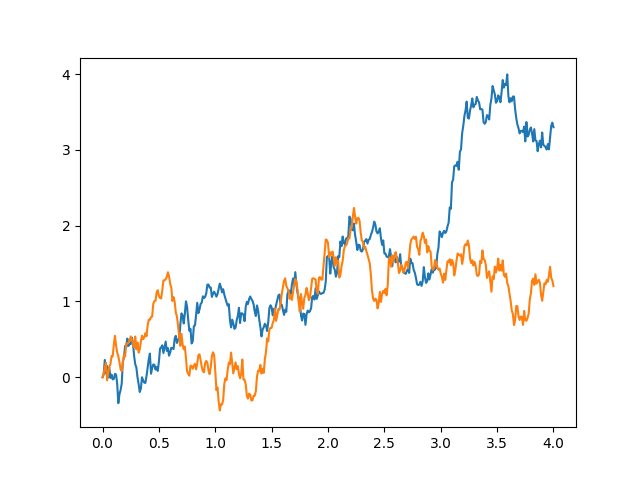
We continue this process, stitching together a path of our Brownian motion, increment by increment.

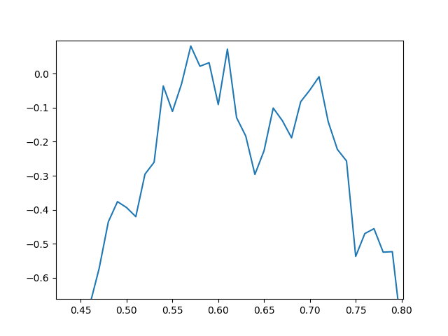
Notes: This is only a simulation, so some key properties of Brownian motion are missing. In theory, if we zoomed in appropriately, the path should look the same on this smaller scale, equally jagged as the wider view. It behaves like a fractal. However, this is clearly not the case in our simulation. When we zoom in it is clear our graph is just made up of line segments connecting the endpoints of the intervals.

My code is far from elegant, but I intend to update with a more general tool to simulate a general Ito Process. For now, here is what I used.